This Atmospheric Model app uses a simple radiative transfer model for a planet with two leaky* atmospheric layers. It begins by calculating Te, the emission temperature of the planet by using the Solar constant and planetary Albedo. Te is called the Blackbody temperature because it is inferred by fitting a Blackbody curve to the observed outbound LWIR radiation.
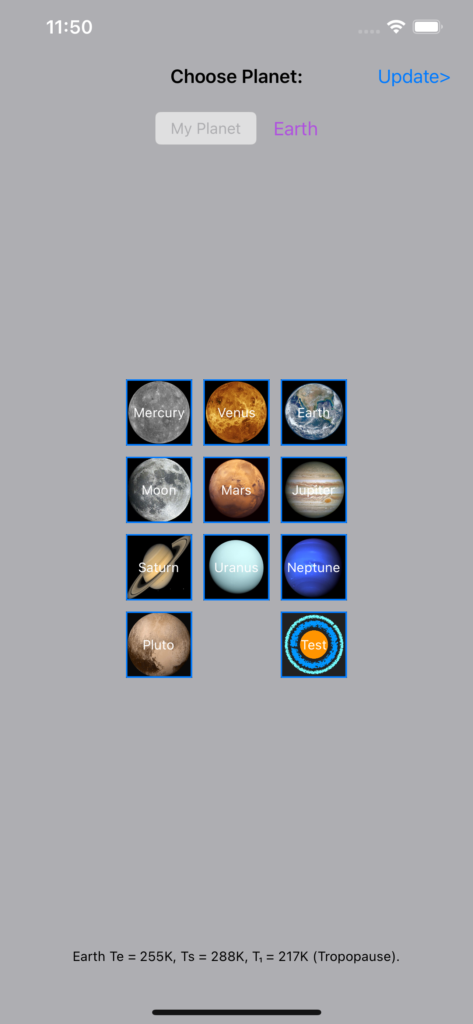
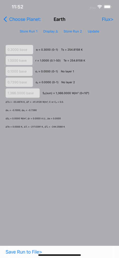
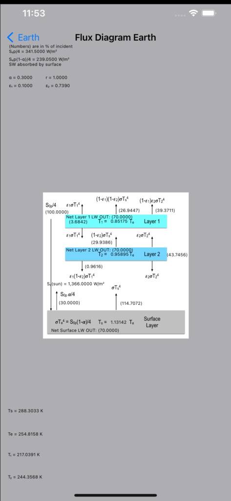
You can choose any of the 9 planets in our solar system, or choose one of your own making. The app then uses 5 parameters for the chosen “base” planet: the Albedo (α), distance from the sun (r), extinction coefficients of two atmospheric layers (ε1, ε2), and the solar constant S0 to calculate temperatures and radiative flux densities. One can modify these 5 adjustable parameters from their base values, and update the result. A flux diagram is generated showing the incoming short wavelength (SW), and outgoing long wavelength (LW) radiation. Two model run results can be saved and differences displayed. Also, runs can be saved to a .csv file for E-mail export and spreadsheet analysis.
Calculate the “natural” 33K greenhouse effect (compare Earth with and without an atmosphere), or change the extinction coefficients to see the effect of adding or reducing absorbing gasses. Predict what Mars might be like with an atmosphere, or see what would happen if the characteristics of our sun, albedo or planetary orbit change. Our sun’s luminosity will increase ~10% in the next billion years.
This simple model can create hours of fun but realize it cannot generate the surface temperature (Ts) of Venus. It’s > 96% CO2 atmosphere would require N = (Ts/Te)4 -1 = 110 fully absorbing atmospheric layers to predict it’s Ts of 737K. However, the base parameter values for Earth nicely calculate Ts, Te, and T1 (upper troposphere) values, and the model correctly predicts Te’s for all the planets.
INSTRUCTIONS:
Load Atmospheric Model app, choose a “base” planet, segue with Update.
Click Update to calculate the temperatures and flux densities.
Segue to inspect the flux densities, and/or modify the base parameters to see changes.
Save and compare differences in 2 runs. (C/C0) values are in CO2 equivalents.
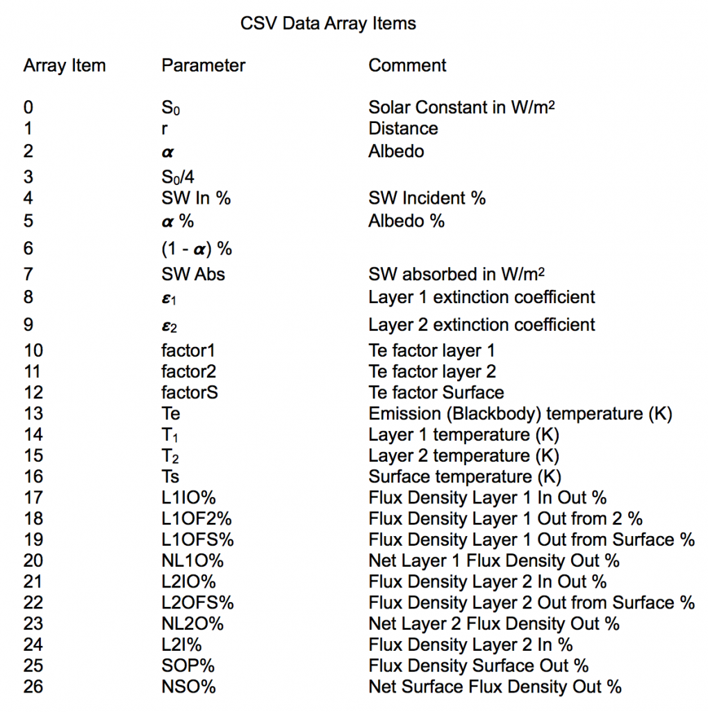
Save runs to .csv file for spreadsheet analysis.
USAGE TIPS:
Start with a base planet, but remember this 2 layer model cannot accurately predict the surface temperatures of the gas giants or Venus.
Pressing the Back button allows you to refresh your parameter or base planet choices.
Remember an ~ 5 K change in Ts resulted in the Earth’s last Ice Age!
For convenience, the Test planet can be used to create your own set of parameters without entering a planet name.
Increasing the solar constant increases all temperatures. Increasing ε does nothing to Te, which depends only on S0, r, and α.
Press On/Off & Home takes flux diagram screenshot.
It is easy to remove a saved data file run (row) after import to spreadsheet.
Atmospheric Model – Version 1.01 12/17/17 – What’s New in this version: Pinch, pan, and double Tap (restore) gestures added to Update and Flux views for better iPhone visibility. Minor bug fix.
RADIATIVE FORCING and CLIMATE SENSITIVITY:
Radiative forcing (ΔF) can be used to estimate the change in surface temperature (ΔTs) arising from that forcing using:
ΔTs = λ x ΔF, where λ is the Climate Sensitivity in K / (W/m2).
Forcing due to an atmospheric greenhouse gas such as CO2 can be expressed as:
ΔF (in W/m2) = 5.35 × ln (C/C0), where C is the CO2 concentration [CO2] and C0 is the initial concentration (in ppm).
For a doubling of [CO2] ΔF = 5.35 x ln (2) = 3.71 W/m2. An IPCC assessment reported that such a forcing (including feedbacks) would result in a ∆Ts of 3 ± 1.5 K. Thus a value for Climate Sensitivity would be (3 ± 1.5) / 3.71 = λ = 0.8 ± 0.4 K/(W/m2).
For a single atmospheric layer Earth, changing the base value of ε = 0.78 to ε = 0.83 (∆ ? = 0.05) gives an ~ 3K T rise; roughly the equivalent of doubling [CO2] (and a forcing of 3.71 W/m2).
There has been a [CO2] increase between the years 1750 (280 ppm) and 2000 (380 ppm). Thus ∆F = 5.35 x ln (370/280) = 1.5 W/m2. ΔTs = λ x ΔF = 0.8 (K/(W/m2)) x 1.5 (W/m2) = 1.2 K over that timeframe (∆ ε ~ 0.02 used).
* Leaky implies ε < 1.